Last year Will Cadell wrote Geospatial Analytics Will Eat The World, And You Won’t Even Know It With this in mind I will describe and illustrate 13 basic GIS analysis tools. The world doesn’t need to know these tools, but every GIS practitioner is advised to master them.
Introduction
About 2 years ago I wrote the article 5 Types of Questions GIS Can Answer. As a recap here are the types of questions that I discussed:
- Where is it? – find locations or features that satisfy one or several conditions.
- What is at? – view and query map layers in a given location or geography.
- What has changed? – study the change in spatial phenomena over time.
- What patterns/relationships exist? – find areas of similarity and discover relationships within your data.
- What if …? – use spatial modeling to predict the outcome of actions and interventions.
Two years down the line I have realized that GIS doesn’t have all the answers and is best used in combination with other technologies. So rather than reviewing the earlier article, I decided to discuss and illustrate some unique and powerful GIS capabilities.
The GIS capabilities that we will review are taken from the Analysis Tools toolbox in ArcGIS Pro. The toolsets that we will explore are Extract, Overlay and Proximity. The illustrations that demonstrate how the tool works have been prepared in ArcGIS Pro with a variety of local datasets.
I used ArcGIS Pro, but you will find similar analysis tools in popular GIS software packages like QGIS. They could have a different name or work slightly differently.
Extract Tools
These tools create new subsets from existing feature datasets by reducing the logical content or geographic extent. The tools can be used in combination to create just the datasets that you need within a given project or analysis workflow.
Select
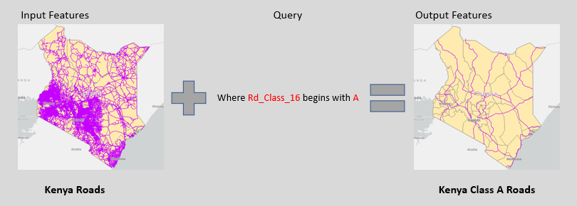
The Select tool creates a subset of the Input Features using a logical expression in the form of an SQL statement. In the example below we select the Class A roads from the Kenya Roads Board dataset using the begins with operator in the Query Builder.
From the output features we can easily identify the Class A roads crossing into Kenya’s neighboring countries. This information can inform the addition of border crossings or the enhancement of cross-border trade at the existing locations.
Clip
The Clip tools acts like a cookie cutter and extracts Input Features that are within the extent of the Clip Feature(s). In the example below we use Machakos County as a cookie cutter to extract the roads within Machakos County into a new dataset.
Clip is probably one of the most widely used GIS tools, since it helps to reduce larger datasets to the extent of your study area. For Machakos County the output features can be used to calculate the length of their road network and identify areas where roads must be constructed or upgraded.

Split
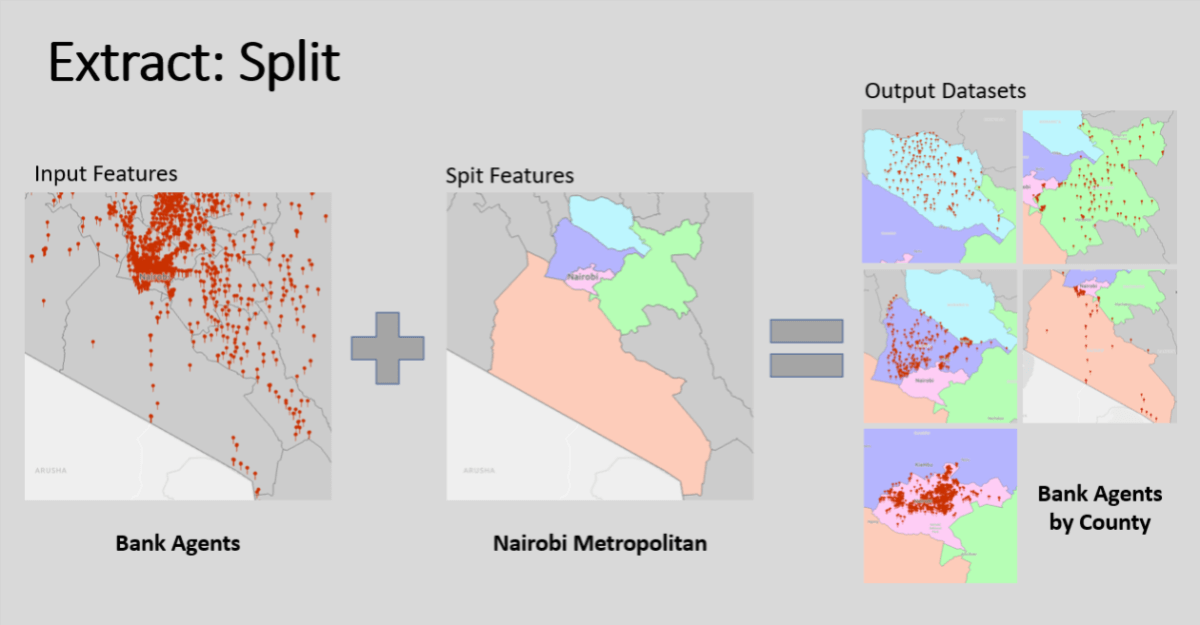
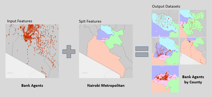
The Split tool splits the Input Features into several output datasets (or tiles) based on an attribute in the Split Features dataset. In the example below bank agent locations from FSK Kenya are split into five subsets using the counties within the Nairobi Metropolitan area as the Split Features.
The Split tool can be used to geographically disaggregate your data. So, a Kenya dataset can be broken down into 47 county datasets. In a similar fashion you could use a grid reference to decompose a larger area into a collection of map sheets.
Overlay Tools
GIS datasets and layers are vertically integrated by a common location reference. This concept enables overlay functions to create new datasets from existing datasets using feature coincidence. The tools that we will review might remind you of set theory and logical operators.
Intersect
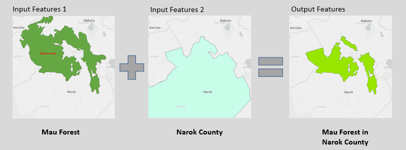
The Intersect tool computes the geometrical intersection of any number of input feature datasets and is equivalent to the logical AND operator. The example below computes the section of Mau Forest within Narok county as the intersect between Mau Forest and Narok County.
Intersect is most frequently used on polygons, but it can be used to find coincidence between point, line and mixed features. Intersect is invaluable in multi-criteria decision-making when you need to find locations that satisfy multiple conditions.
Union
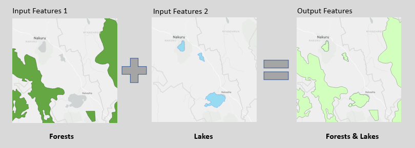
The Union tool computes the geometrical union of any number of input feature datasets and is equivalent to the logical OR operator. The example below combines forests and lakes in part of Kenya’s Rift Valley into a dataset that represents vulnerable natural resources.
Union only works with polygons. It can be used to combine datasets with a common theme as shown in our example. Alternatively, it can be used to join datasets collected by different agencies or under different projects.
Symmetrical Difference
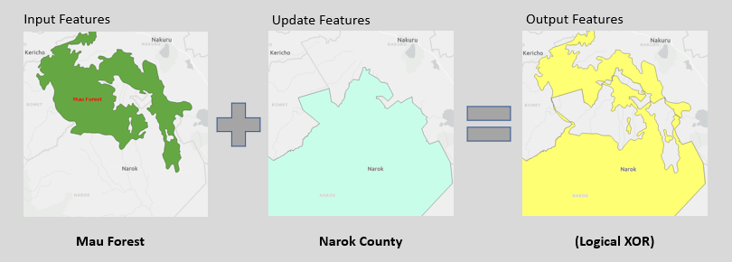
Symmetrical Difference identifies the portions of features in the Input Features and Update Features that do not overlap and is equivalent to the logical XOR operator. The Output Features may appear in either of the datasets, but not in both.
Symmetrical Difference can be used in multi-criteria decision-making when you want either condition to be true rather than both. The example that we’ve used here shows that Narok County and Mau Forest aren’t coincident, but I reckon most of you already knew that.
Erase
The Erase tool removes portions of the Input Features that are coincident with the Erase Features from the Output Features dataset. In the example below we have removed the portion of Homa Bay County that is coincident with Lake Victoria.
The resulting dataset now only contains the land area of Homa Bay County. Erase is a powerful complement to Intersect in multi-criteria decision-making. For example, you could use it to exclude wetlands and forests from open areas that are considered for urban development.

Identity
The Identity tool computes the geometric intersection of the Input Features and Identity Features and combines their attributes in the Output Features dataset. The Input Features can have any geometry type, but the Identify Features must be polygons or have the same geometry type.
In the example below Identify has been used to calculate the geometric intersection and combined attributes of Mau Forest and the counties that it covers. The output dataset contains the sections of Mau Forest that fall within the jurisdiction of Narok, Nakuru, Bomet, and Kericho.

Update
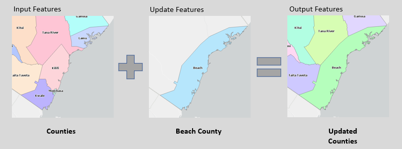
The Update tool calculates the geometric intersection of two datasets and updates the Input Features with the Update Features to create the Output Features dataset. In the example below the existing Counties of Kenya are updated with a newly formed Beach County.
Update comes in handy when a section of a large datasets needs to be updated with newly collected data. Consider updating a town map with estates that are newly built or upgraded or a land use map that needs to be updated due to drastic land use changes.
Proximity Tools
One type of question that gets asked frequently in GIS is what features are near to one another. The Proximity toolset has a number of tools to determine the proximity of features within or between feature classes.
Buffer
The Buffer tool creates buffers around the Input Features using a fixed or variable buffer distance derived from a feature attribute. The Output Features may be dissolved to create a single polygon. In the example below a 50-meter buffer polygon was created around major roads in Nairobi’s CBD.
From the example we can visually identify structures that are within 50 meters from the centerline of a major road. The buffer polygon could also be used to select building footprints within the buffer zone use Intersect, or any other suitable GIS tool like Spatial Join.

Multiple Ring Buffer
Multiple Ring Buffer creates multiple buffers at specified distances around the Input Features. The output buffers can be merged and dissolved to create non-overlapping buffers. In the example below buffers of 10, 20, 30, 40, and 50 km have been created around the center of Nairobi.
Using the Output Features, we can now quickly estimate the straight-line distance from Nairobi to neighboring towns. For example, the distance to Kiambu is about 15 km and the distance to Thika is about 40 km. It also appears that Limuru is farther from Nairobi’s CBD than Ruiru.

Near
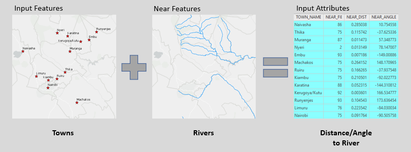
Calculates distance and additional proximity data from the Input Features to the nearest features in the Near Features. The data is written to the attribute table of the Input Features. In the example below proximity data for the nearest river is written to the Town attribute table.
Input Features and Near Features can be of any geometry type, so the Near tool is quite versatile and has many applications. For instance, you can use it to calculate distance and direction from your house to the nearest ATM, highway, or park.
Thiessen Polygons
Thiessen Polygons constructs areas of influence around point features. Any point in a Thiessen polygon is closer to its associate point than to any other point. In the example below Thiessen polygons have been constructed around major towns in Kenya.
The Thiessen Polygons form a Voronoi diagram, which can be used to identify the closest cell tower, hospital, petrol station or retail outlet for any point in a given area. Large Thiessen polygons represent large service areas and can be used to prioritize new service locations.

Wrapping Up
We have looked at 13 basic GIS analysis tools that are available in ArcGIS Pro and many other GIS software packages. These tools can be used and combined to answer different types of questions and solve a variety of problems. Here’s a quick recap:
- Extract tools are used to create subsets of larger datasets. Typically, these tools are used at the start of a GIS workflow or project to prepare just the data that you will need.
- Overlay tools create new datasets from existing datasets using the concept of coincidence. Many of these tools are essential in multi-criteria decision-making and support a variety of GIS workflows.
- Proximity tools created new datasets from existing datasets using the concept of distance. These tools determine which features are near to one another and the results are often used in subsequent analysis.
There are many more GIS analysis tools in addition to the ones that are presented here. Perhaps we’ll review in subsequent articles. Meanwhile start practicing and using the tools that we covered to do some great work.
